There was a question posted on the physics subreddit asking how high in the air a bullet would go if you shot it straight up. It was later removed by the moderators (who knows why?), but I thought it was a good question that would make a good example problem. Normally I would use MATLAB to solve something like this, but I thought it would be a good opportunity for me to start using python more to solve technical problems like this.
In terms of an actual physics problem, here’s how I would state it: a bullet of known dimensions and mass is fired straight upward at a known velocity. What is it’s maximum height, and how long does it take it to get there?
So how do we model this? Once the bullet leaves the muzzle of the gun, there are only two forces acting on it: gravity, and air resistance. Newton’s 2nd law tells us that the acceleration of an object is proportional to the force acting upon it, or in equation form \(F=ma\). The acceleration is defined as the derivative of the velocity with respect to time, or \(a=\frac{dv}{dt}\). So we can write this as a differential equation for the velocity of the bullet as a function of time:
$$m\frac{dv}{dt}=-F_g – F_d$$
Where \(m\) is the mass of the bullet, \(v\) is the velocity, \(t\) is time, \(F_g\) is the force of gravity, and \(F_d\) is the drag force due to wind resistance. This also requires an initial condition for \(v\) at \(t=0\), which is simple the muzzle velocity of the bullet.
The gravitational force \(F_g\) is pretty straightforward: \(F_g=mg\), where \(g\) is the gravitational acceleration of 9.8 m/s2. The drag force is a bit more complicated though. It’s given as
$$F_d=\frac{1}{2}\rho v^2 A C_d$$
Where \(\rho\) is the density of the fluid it’s traveling through (air), \(v\) is of course the velocity, \(A\) is the cross-sectional area of the object (in this case the circular cross-sectional area of the bullet as you look at it head-on), and \(C_d\) is the drag coefficient of the object.
Determining the drag coefficient is what makes this problem a bit complicated. It’s defined as follows:
$$C_d = \frac{2 F_d}{\rho v^2 A}$$
So you can see it’s just a rearranged version of the drag force itself. This appears to be self-referential, but it’s not: the drag coefficient is measured experimentally or by performing fluid dynamics simulations, and it then becomes a function of velocity that we can use for solving other problems.
So we just need to find some results that someone else has already measured experimentally. An internet search found this info sheet, which shows a typical bullet drag coefficient as a function of the Mach number. The Mach number is just the ratio of the velocity of an object to the speed of sound, so if we know the speed of sound in air (we can look this up) then we can use that data to calculate our drag coefficient as a function of velocity.
However this is just a data table on a website. How do we get this into either a functional form or a lookup table that we can use? I was able to find the plot by itself as a separate image:

Then I used the very handy website WebPlotDigitizer to convert it to a csv file. With that in hand we now have everything we need to calculate the trajectory of the bullet. You can download a copy of the csv file for yourself it you want to look at it or use it with the python code I have at the end of this post.
For the actual gun and bullet, I decided I might as well go big: I looked up the parameters for a .50 caliber rifle and ammunition:
| Parameter | Value |
| muzzle velocity | 884 m/s |
| bullet diameter | 13 mm |
| bullet mass | 43 g |
From the bullet diameter we can calculate the cross-sectional area of the bullet \(A\) to be 1.327 cm2.
We’ll need a few other constants as well:
| Constant | Value |
| gravitational acceleration | 9.80665 m/s2 |
| density of air | 1.225 kg/m3 |
So that should be everything we need to solve for the velocity. We also want to solve for the height of the bullet at the same time, fortunately the equation for this is very simple. Since velocity is defined at the derivative of position as a function of time, our second equation then is simply
$$\frac{dx}{dt}=v$$
Where \(x\) is the position/height of the bullet as a function of time. The initial condition is very simple as well, simply \(x(0)=0\).
With this we should have all the information we need to solve for the bullet trajectory. To solve them numerically we’ll need some code that can solve an initial-value problem (ivp). Algorithms to do this are implemented in just about every mathematics software that’s out there: Matlab, Mathematica, Maple, MathCAD, etc. As an exercise I decided to solve this using python, as I’ve been trying to migrate from using Matlab to using python more. We’ll need the equations written out in matrix form to be able to solve them numerically:
$$\mathbf{y}= \begin{bmatrix} x \\ v \end{bmatrix}$$
$$\frac{d\mathbf{y}}{dt}= \begin{bmatrix} v \\ -g-\textrm{sgn}(v)\frac{1}{2}\frac{\rho}{m} v^2 A C_d(v) \end{bmatrix}$$
$$\mathbf{y}(0)= \begin{bmatrix} 0\\ v_0 \end{bmatrix}$$
We need the sign function \(\textrm{sgn}(v)\) so that air resistance is always resistive: in other words it has to act against the direction of the velocity. If we just kept it as a minus sign, it would work correctly when the bullet is traveling upward, but when it switches to moving downward it would instead accelerate it downwards. This ensures that air resistance will always slow the bullet down, regardless of whether it’s moving up or down.
Solving those equations (I’ll share the code at the bottom of this post) we get the following curves for the bullet height and velocity:
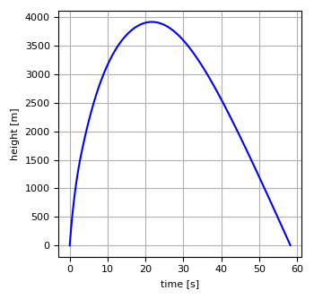
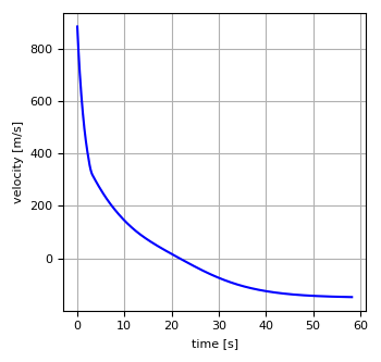
The bullet reaches a maximum height of 3917.4 m in 21.70 s. It then impacts the ground at a velocity of 147.7 m/s at 58.27 s. You can see that the bullet took a lot longer to hit the ground after falling form the apex than it did to get there, because drag had slowed it down a lot by that time. Also you can see that by the time the bullet is hitting the ground that the velocity curve is almost completely flat, indicating that the bullet has just about reached its terminal velocity.
So the next question is, are all of our assumptions valid? The bullet is traveling almost 4 km into the air, and we know that the air gets thinner as we go higher in altitude. The drag is proportional to the density of the air, so that means there should be less air resistance at higher altitudes.
Can we calculate the density of the air as a function of the height of the bullet? Yes, we can! Wikipedia is our friend here, as it has the exact equation we need:
$$\rho=\frac{P_0 M \left( 1-\frac{L x}{T_0} \right)^{\frac{gM}{Rx} -1}}{R T_0}$$
Where \(x\) is the height above sea level, \(g\) is gravitational acceleration as before, and the other parameters are as follows:
| Symbol | Parameter | Value |
| \(P_0\) | atmospheric pressure at sea level | 101325 Pa |
| \(M\) | molar mass of air | 0.0290 kg/mol |
| \(L\) | temperature lapse rate | 0.0065 K/m |
| \(T_0\) | temperature at sea level | 15°C (288.15 K) |
| \(R\) | universal gas constant | 8.314 J/(K mol) |
There is one other thing to consider: our table for determining the drag coefficient is listed as a function of the Mach number, which is the velocity divided by the speed of sound. Well, the speed of sound also depends on the density and pressure of the air. The specific formula for this is also in Wikipedia. In the end it becomes a function of the temperature:
$$c=\sqrt{\frac{\gamma R T}{M}}=\sqrt{\frac{\gamma R T_0\left( 1-\frac{Lx}{T_0}\right)}{M}}$$
Where \(\gamma\) is the heat capacity ratio, which for air is equal to 1.4.
Adding these corrections to the air density and speed of sound changing as a function of altitude, we get the following solutions for the detailed model compared to the simple model:
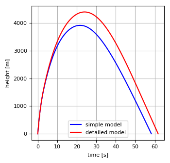
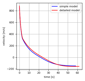
For the more detailed model, the bullet reaches an apex of 4400 m in 24.0 s, and it impacts the ground at a velocity of 155.1 m/s at 61.76 seconds. So as we surmised, the bullet is able to travel higher than predicted with the simple model because at high altitudes the air is thinner and provides less air resistance.
We could also try to account for gravitational acceleration decreasing as we increase in altitude, but at a height of 4 km this is only a 0.1% difference: this is actually smaller than the difference in gravitational acceleration between being at one of the poles and being at the equator: it’s approximately 0.3% less at the equator due to the spinning of the earth, and the earth bulging slightly at the equator. We can safely ignore both of these effects.
So as promised, here is my code. I found a small error that I fixed, it should be working now:
# -*- coding: utf-8 -*-
"""
Created on Wed Dec  2 18:50:14 2020
@author: Derek Bassett
"""
import pandas as pd
import numpy as np
import matplotlib.pyplot as plt
from scipy.integrate import solve_ivp

# parameters
v0 = 2900           # muzzle velocity [ft/s]
v0 = v0*12*2.54e-2  # [m/s]
x0 = 0              # initial position [m]
d = 1.3e-2          # bullet diameter .50 BMG [m]
A = np.pi*(0.5*d)**2 # cross-sectional area [m^2]
m = 0.043           # bullet mass FMJBT-PMC [kg]
tf = 65             # time to end calculation [s]

# constants
g = 9.80665         # gravitational acceleration [m/s^2]
R = 8.31447         # universal gas constant [J/(K*mol)]
M = 0.0289654       # molar mass of dry air [kg/mol]
p0 = 101325         # sea level standard atmospheric pressure [Pa]
T0 = 288.15         # sea level standard temperature [K]
L = 0.0065          # temperature lapse rate [K/m]
gamma = 1.4         # adiabatic index for dry air [1]

def rho_air(h): # calculate density of air as a function of altitude
    rho = ((p0*M)/(R*T0))*(1-(L*h)/T0)**((g*M)/(R*L)-1)
    return rho

def csound(h): # calculate the speed of sound as a function of altitude
    c = np.sqrt((gamma*R*T0*(1-(L*h)/T0))/M)
    return c

# use data from csv for drag coefficient
df = pd.read_csv('drag_coefficient.csv',header=None)
CDarray = df.to_numpy()

def CD_sim(u): # calculate the drag coefficient as a function of velocity and height
    # calculate speed of sound c
    c = csound(x0)
    # calculate Mach number Ma
    Ma = u/c
    # interpolate to calculate the drag coefficient CD
    CD = np.interp(Ma,CDarray[:,0],CDarray[:,1])
    return CD

def CD(u,h): # calculate the drag coefficient as a function of velocity and height
    # calculate speed of sound c
    c = csound(h)
    # calculate Mach number Ma
    Ma = u/c
    # interpolate to calculate the drag coefficient CD
    CD = np.interp(Ma,CDarray[:,0],CDarray[:,1])
    return CD

def yprime_sim(t,y):# simple formulation neglecting change in air density with altitude
    ydot = np.empty(2)
    ydot[0] = y[1]
    ydot[1] = -g - np.sign(y[1])*0.5*(rho_air(x0)/m)*y[1]*y[1]*A*CD_sim(y[1])
    return ydot

def yprime(t,y):# formulation that accounts for the change in air density with altitude
    ydot = np.empty(2)
    ydot[0] = y[1]
    ydot[1] = -g - np.sign(y[1])*0.5*(rho_air(y[0])/m)*y[1]*y[1]*A*CD(y[1],y[0])
    return ydot

# stop simulation when bullet hits ground
def hit_ground(t,y): return y[0]
hit_ground.terminal = True
hit_ground.direction = -1
# determine where velocity=0
def apex(t,y): return y[1]

Y0 = np.array([x0,v0])
t = np.linspace(0,tf,1001)

# solve equations
sol1 = solve_ivp(fun=yprime_sim,t_span=(0,tf),y0=Y0,t_eval=t,events=(apex,hit_ground),dense_output=True)
sol2 = solve_ivp(fun=yprime,t_span=(0,tf),y0=Y0,t_eval=t,events=(apex,hit_ground),dense_output=True)

# plot results
fig = plt.figure(num=0,figsize=(3.5,3.0),dpi=100,facecolor=None,edgecolor=None,frameon=False,clear=True)
plt.plot(sol1.t,sol1.y[0,:],'b-',label='simple model')
plt.plot(sol2.t,sol2.y[0,:],'r-',label='detailed model')
plt.legend(loc='best')
plt.xlabel('time [s]')
plt.ylabel('height [m]')
plt.grid()
plt.tight_layout()
plt.show()
fig.savefig('height02.png',transparent=True)

fig = plt.figure(num=1,figsize=(3.5,3.0),dpi=100,facecolor=None,edgecolor=None,frameon=False,clear=True)
plt.plot(sol1.t,sol1.y[1,:],'b-',label='simple model')
plt.plot(sol2.t,sol2.y[1,:],'r-',label='detailed model')
plt.legend(loc='best')
plt.xlabel('time [s]')
plt.ylabel('velocity [m/s]')
plt.grid()
plt.tight_layout()
plt.show()
fig.savefig('velocity02.png',transparent=True)

print(f'Simple model reached apex of {sol1.y_events[0][0][0]:.1f} m at t={sol1.t_events[0][0]:.2f} s. '+
      f'It impacted the ground at a velocity of {-sol1.y_events[1][0][1]:.1f} m/s at t={sol1.t_events[1][0]:.2f} s.')
print(f'Detailed model reached apex of {sol2.y_events[0][0][0]:.1f} m at t={sol2.t_events[0][0]:.2f} s. '+
      f'It impacted the ground at a velocity of {-sol2.y_events[1][0][1]:.1f} m/s at t={sol2.t_events[1][0]:.2f} s.')
Feel free to copy the code and play around with it.