Brain Stretching of a Spinning Skater

Posted on March 5, 2023 by admin

So I was wasting time on reddit the other day (happens all too often) where I came across the following video of a girl practicing spinning for figure skating using an off-ice apparatus:

You can see the post I read here, there were a lot of comments about how spinning that fast can’t possibly be good for the girl’s brain. My initial response was that since her head is at the center of the axis of rotation there really isn’t any force on it, but technically that’s not true: if you have something soft and squishy and you spin it really fast, it will bulge out in the middle and compress slightly at the top and bottom along the axis of rotation:

Note: thanks to thingiverse for the brain model, and blender for the rendering.

It probably doesn’t stretch out this much. But can we estimate how much it actually does stretch out when someone’s head is spinning around this fast? How would we estimate this? There are three pieces of information we need:

How fast the girl is spinning
Physical parameters of the brain
A model or equation to calculate/estimate the deformation of the brain while its spinning

Speed of Spinning Girl

How can we figure out how quickly the girl is spinning? This should be fairly straightforward with some video analysis. Analyzing the video the way we need to though, requires us to be able to scan the video one frame at a time, and have a timestamp for each frame. Then we can start at the point in the video where the skater is spinning the fastest, walk through several rotations, and count the time elapsed by comparing timestamps. Then the rotation speed is simply # of rotations / time elapsed.

I don’t have any expensive video editing/analysis software, but a quick google search for a free open source software for basic video editing led me to Avidemux.

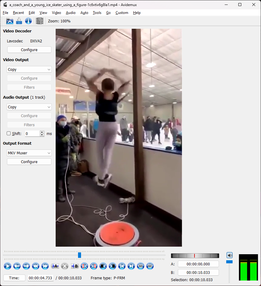
The software lets me step through one frame at a time with the Left and Right keys, and gives me a timestamp at the bottom. More than sufficient for my needs. Starting at 4.733s and ending at 7.833s, she goes through 14 rotations. That comes out to 4.52 revolutions/s.

Mechanical Properties of the Brain

Doing a quick google search for the mechanical properties of the brain almost gave me too much information, there were hundreds of academic papers discussing it. I ended up using this paper: Biomechanical Modeling of Brain Soft Tissues for Medical Applications. It gives values across a range of values from other studies, but I ended up going with a lower-end value (since that will give a larger deformation) of Young’s modulus E = 2 kPa, and Poisson’s ratio of ν = 0.45. For density we’ll just assume it’s about the same as water, since it’s soft tissue and our body is after all mostly water, so that’s a density of 1000 kg/m³.

Deformation Model

This was actually a bit harder for me to find. Searching for “deformation of rotating elastic sphere” and other similar search terms got me lots of papers and pages showing how the earth (or some other planet) bulges at the center due to its spin. However in that case the restoring force trying to return it back to being spherical is gravity, while in our case for the spinning brain it’s simply the object’s own elasticity.

Eventually I was able to find an online solid mechanics textbook that had the derivation for the elastic deformation of a spinning circular plate. Sure, it’s not quite the same as a sphere, but for our intents and purposes we can approximate the brain as a cylinder as much as we can a sphere. For the displacement of the cylinder/disc it gives the following equation:

$$\mathbf{u}=(1-\nu) \frac{\rho \omega^2}{8E} \{ (3+\nu)a^2 r – (1+\nu)r^3 \}\mathbf{e}_r – \nu \frac{\rho \omega^2 z}{8E} \{ 2(3+\nu)a^2 – (3\nu +2)r^2 \}\mathbf{e}_z$$

That’s given in vector form, so since we’re only interested in deformation in the r direction at at the very edge where $r=a$, we can simplify it to the following:

$$u_r(a) = \frac{\rho \omega^2 a^3}{4E} (1-\nu)(3-\nu)$$

The only parameter we’re missing is the radius of our cylinder. A quick google search tells me that the average human brain has a volume of 1400cm³. If we approximate the brain as a cylinder with equal height and diameter, we can calculate the radius using the following derivation:

$$V = \pi r^2 h = \pi r^2 (2r) = 2 \pi r^3$$

$$r = \left( \frac{V}{2 \pi} \right)^{1/3} = \left( \frac{1400 \text{cm}^3}{2 \pi} \right)^{1/3} = 6.0 \text{cm}$$

We also need to convert our rotation speed to radians/s, which is just multiplying rotations/s by $2 \pi$ which gives us $\omega = 28.38 \text{/s}$.

So our final calculation is:

$$u_r(a) = \frac{(1000 \text{kg}/\text{m}^3) (28.38 \text{/s})^2 (0.06 \text{m})^3}{4 (2000 \text{Pa})} (1-0.45)(3-0.45)=0.03 \text{m} = 3.0 \text{cm}$$

Well, that is a very large displacement, our brain is stretching from a 12cm diameter to 18cm! Now there are some problems that this result indicates:

Our model assumed a simple perfectly elastic solid. In reality this assumption only holds for small deformations, after a certain amount of displacement it ceases to be elastic (i.e. if you relieve the stress then it returns to its original shape) and becomes plastic deformation (i.e. the shape permanently changes), etc.
The brain is encased in the cranial cavity, and doesn’t have very much room to stretch. The gap between the brain and the cranium is 0.4mm to 7mm depending on the location.

Now if the maximum displacement had been < 0.1mm or so (which is what I assumed) it wouldn’t really make a difference, those assumptions would have been fine. But with this kind of a predicted large displacement we can’t use such a simplified model any more.

But wait! Maybe it isn’t the model itself that’s bad, but the boundary conditions! When solving for the equation for $u_r(a)$ above, we make the assumption that the radial stress is zero at $r=a$. However if the brain is constrained inside the cranial cavity so that it can’t expand, then a better boundary condition would be that the displacement $u_r(a)=0$. This won’t give us much (if any) displacement inside the brain, but we can still calculate the stress inside the brain material.

Redoing the derivation, we start with our differential equation:

$$\frac{\partial}{\partial r}\left( \frac{1}{r} \frac{\partial}{\partial r} (ru) \right)=-\frac{1-\nu^2}{E}\rho \omega^2 r$$

Integrating twice gives us the displacement $u$ with the integration constants $A$ and $B$:

$$u=-\frac{1-\nu^2}{8E}\rho \omega^2 r^3 + Ar + \frac{B}{r}$$

The solution has to be finite at $r=0$, so that means $B=0$. To solve for $A$ we set the condition that the displacement has to zero at the edge, or $u(a)=0$. That gives us a formula for the displacement:

$$u(r)=\frac{1-\nu^2}{8E}\rho \omega^2 (a^2 r-r^3)$$

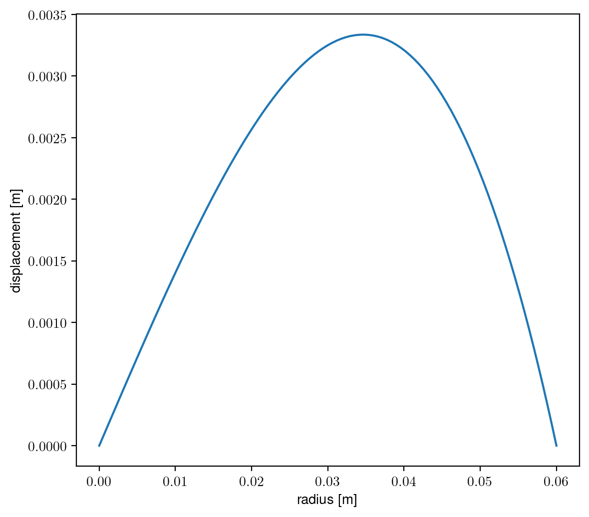
So our cylinder model of a brain is displacing a maximum of about 3mm around halfway between the center and the edge. A more general dimensionless version of the plot is here:

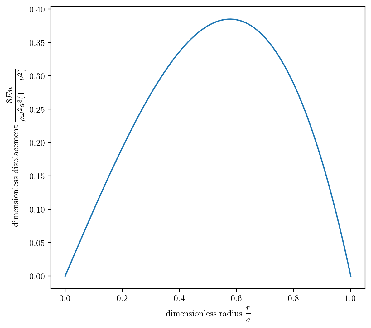
This is a more general version of the solution which is valid for any size cylinder with any known parameters of Young’s modulus $E$, density $\rho$, rotation speed $\omega$, radius $a$, and Poisson’s radio $\nu$.

Another thing we can calculate is how much stress there is inside our cylindrical brain as a function of radius.

$$\sigma_{rr}=\frac{E}{1-\nu^2}\left( \frac{\partial u}{\partial r} + \nu \frac{u}{r} \right)$$

Substituting in our derived function for $u$ we can simplify it to the following function:

$$\sigma_{rr}=\frac{\rho \omega^2}{8}\left( a^2(1+\nu) – r^2(3+\nu) \right)$$

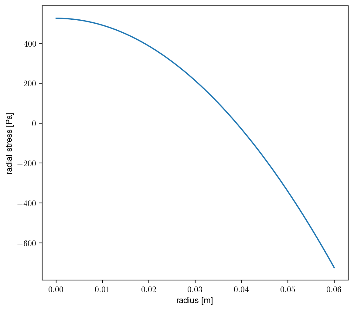
This shows that the ‘brain’ is stretching in the center (positive stress), and being compressed at the edge (negative stress).

I tried to look up how much mechanical stress a human brain can withstand, but it’s almost impossible to filter out psychological stress from search results, and everything else is about sudden shocks to the brain: concussions, CTE, etc.

I found a few papers talking about different types of brain injury:

S. Kleiven, X. Li, A. Eriksson, and N. Lynøe, “Does High-Magnitude Centripetal Force and Abrupt Shift in Tangential Acceleration Explain High Risk of Subdural Hemorrhage?,” Neurotrauma Reports, vol. 3, no. 1, pp. 248–249, Jan. 2022, doi: 10.1089/neur.2022.0025.
B. D. Stemper et al., “Head Rotational Acceleration Characteristics Influence Behavioral and Diffusion Tensor Imaging Outcomes Following Concussion,” Ann Biomed Eng, vol. 43, no. 5, pp. 1071–1088, May 2015, doi: 10.1007/s10439-014-1171-9.
S. Kleiven, “Why Most Traumatic Brain Injuries are Not Caused by Linear Acceleration but Skull Fractures are,” Frontiers in Bioengineering and Biotechnology, vol. 1, 2013, Accessed: Mar. 05, 2023. [Online]. Available: https://www.frontiersin.org/articles/10.3389/fbioe.2013.00015

The second one is specifically related to rapid rotational acceleration, as opposed to impacts which is what almost everything else is. But it’s specifically about acceleration, where in our video the girl isn’t really accelerating that quickly in her rotational motion, even if her rotational velocity is quite high.

So ultimately a bit inconclusive in this post, though I was able to learn a lot about solid mechanics and deformation.

Posted in Science | Tagged centrifugal force, figure skating, solid mechanics | Leave a comment

Cost/benefit analysis of martial arts training and self defense

Posted on January 15, 2022 by admin

I was thinking about my history of training martial arts and how it’s worth/benefit would be analyzed from a purely dispassionate/rationalist perspective. Many (possibly majority) of people start learning martial arts for self defense: i.e. to (hopefully) learn how to protect themselves if they are ever in a life or death violent situation. How well does learning martial arts actually do this? Can we analyze it from a quantitative point of view?

One simple way we could analyze would be to use the following equation:

$$[\text{Value}] = [\text{Benefits}]-[\text{Costs}]$$

Pretty simple. If our total benefits are greater than our total costs, it will be a positive value. So what are we exactly measuring here? Lets say time, as in lifespan. If someone attacks me and I die, then my total lifespan is shorter than if I successfully defend myself and am able to live longer. The associated cost in time would be the time spent training martial arts.

So how do we calculate or at least estimate the increased lifespan? I would formulate it like this:

$$[\text{Gained Lifespan}]=(Y-A)p$$

Where $Y$ is the average lifespan for your demographic (currently 79 years in the U.S.), $A$ is your current age (for sake of argument we’ll say 20 years old), and $p$ is probability that you encounter a situation where your martial arts training makes the difference between life and death or serious injury.

However, that equation isn’t quite right. It is the gained lifespan if I were attacked and am able to save myself right when I am 20 years old, in which case I would gain 59 years of life. But if I were attacked when I was 78 years old, on average I would only gain one additional year of life. So we need to take it from the average age I would be, which is just the half-way point between $Y=79$ years and $A=20$ years, so the corrected equation is:

$$[\text{Gained Lifespan}]=\frac{Y-A}{2}p$$

As for $p$, we currently have no idea what that probability could be, so let’s leave it for now.

The time cost is pretty easy to calculate. Let’s say you study martial arts for 10 hours/week for 10 years. The total time spent learning is then:

$$[\text{Time Cost}]=C=(10\; \text{hr}/\text{wk})(52\; \text{wk}/\text{yr})\left( \frac{1 \;\text{day}}{24\; \text{hr}} \right)\left( \frac{1\; \text{yr}}{365\; \text{day}} \right)(10\; \text{yr}) = 0.59\; \text{yr}$$

At this point we know every term in the equation to calculate $[\text{Value}]$ but the probability $p$. What we can do though is calculate what $p$ would have to be for us to break even, i.e. the point where the the expected or average gained lifespan is equal to the time we spent learning the martial arts in the first place. That’s simply setting $[\text{Value}]=0$ and solving for $p$. Doing so we get:

$$p=\frac{2C}{Y-A} = \frac{2 (0.59\;\text{yr})}{79 \;\text{yr} -20 \;\text{yr} }=0.02$$

So our final probability is $p=0.02$ or 2%. If our martial arts training is able to save our lives when we are in a life-threatening situation, then it’s worth it to spend 10 hrs/week training for 10 years if there is at least a 2% of us being killed by violence before we die of natural causes.

So what is the chance of us being killed? In the US, the CDC states that currently there are 5.8 homicides per 100,000 people per year. So assuming that homicides are completely random (which of course they aren’t, but for the sake of argument we’ll go with that simplification), then we have a $p=0.000058=5.8 \times 10^{-5}$ probability or a 0.0058% chance of being killed by homicide in any given year.

But we need to know the total probability of it happening over the course of $Y-A=59$ years, not just one! How do we calculate that? We can’t just add them all up 59 times and say the total probability is $P=59p$, since you can’t just add up probabilities like that. That’s like saying if you roll a 6-sided die six times that you’re guaranteed to roll 6, or if you flip a coin twice you’re guaranteed to get a heads. And we can’t multiply $p$ by itself 59 times either, $P=p^{59}$ is the probability of someone being killed ever year for 59 years! Of course you can only be killed once (that we know of), but even if you could be killed more than once it becomes an astronomically small chance.

What we do is instead calculate the probability that we aren’t killed in 1 year, multiply that by itself 59 times to get the probability we aren’t killed at all over 59 years, and then subtract that by 1 to get the probability that we would be killed over 59 years.

$$P = 1-\left( 1-p \right)^{Y-A}=1-\left( 1- 5.8 \times 10^{-5} \right)^{59} = 0.0034$$

Or a 0.34% chance of a person being killed over the course of 59 years. That’s pretty high (3 people in 1000), but it’s still much smaller than the 2% required for our martial arts training to be ‘worth it’ from a cost/benefit analysis perspective.

However all this analysis invites an obvious question: would this 10 hrs/week of training for 10 years actually give me the skills to protect myself if I were to be violently attacked by someone? Does it even make any difference?

In terms of a deadly assault where someone is attacking you with a knife or a gun, I’m afraid the answer is: probably not. Statistically it’s hard to evaluate this. Lots of martial arts claim to be able to teach people to defend themselves against an attacker with a knife or a gun (and I’ve trained some of them myself), but unfortunately this isn’t very realistic. If someone has a gun on you and they intend to kill you, it’s very difficult to survive. Similarly if someone has a knife on you and intends to slash and stab you, your chances of getting out without a serious or fatal injury is very difficult.

This second scenario is actually pretty easy to test in relative safety with a partner. Put on a fairly close-fitting shirt and pants (that can get stained), and the attacker has a large permanent marker to simulate a knife. The attacker’s goal is to mark your body with the magic marker as many times as they can, and the defender’s goal is to take the marker away from them without getting any marks on them. You’ll find it’s pretty much impossible, even for a skilled martial artist, to be able to successfully defend themselves even against a relative beginner without several marks on their clothing, often in very dangerous areas (torso, thigh, wrist, neck, etc.)

You can do the same type of thing with a paintball gun and some protective equipment, but it can get a lot more messy. The results are pretty much the same though: the odds of the defender not being killed or seriously injured/maimed are very small.

Some of the best realistic conversations on this I’ve seen on the internet are by a couple of guys that evaluate some of the least realistic fight scenes on film: Logan Lo and Chad Vasquez at the Scenic Fights YouTube channel. These guys have a lot of experience doing full-contact martial arts with full resistance and with weapons, and they have a lot of great commentary on what is or is not realistic in a combat situation, and the realistic portrayal of fighting someone with or without a weapon.

Whether you should fight back or not can depend on a lot of different factors. A drunk belligerent guy in a bar pushes you? De-escalate and walk away. Someone with a gun or a knife demands your wallet? Just give them your wallet. Several dudes with baseball bats start approaching you menacingly? Just run and hope you can get somewhere safe. But someone with a gun tries to get you into a car? Statistically the odds of you getting out alive aren’t good, you should probably resist and fight back. Someone takes a swing at you? Combat has already started, it’s hard to get out of it at that point and you need to defend yourself. So basically, context matters.

So how likely is an assault to become a murder? Is there any data that we can use to estimate this? A couple of searches got me to these two sites: number of aggravated assaults in the US in 2020, and number of homicides in the US in 2020.

Here is a python Jupyter notebook with the data and plots:

Assault and Murder Statistics 2020

In [33]:

import matplotlib.pyplot as plt
import numpy as np

assaults = {"Personal":74403, "Handgun":69423, "Knife":61924, "Blunt":39643, "Firearm":39548, "Asphyxiation":10640,
           "None":8346, "Unknown":7772, "Rifle":4892, "Shotgun":2948, "Handgun(automatic)":2862, "Other Firearm":2646,
           "Firearm(automatic)":943, "Fire":865, "Poison":485, "Drugs":456, "Rifle(automatic)":287, "Explosives":250,
           "Other Firearm(automatic)":82, "Shotgun(automatic)":38, "Other":29497}
assaultsKeys = assaults.keys()
assaultsValues = assaults.values()
#plt.bar(assaultsKeys,assaultsValues)
#plt.xticks(rotation='vertical')
y_pos = np.arange(len(assaultsKeys))
plt.figure(figsize=(8,10))
plt.barh(y_pos,assaultsValues, height=0.8, align='center')
plt.yticks(y_pos,labels=assaultsKeys)
plt.gca().invert_yaxis()
#plt.xscale('log')
plt.title('US Assault Crimes in 2020')


murders = {"Handgun":8029, "Firearm":4863, "Knife":1739, "Personal":662, "Rifles":455, "Blunt":393,
           "Shotgun":203, "Other guns":113, "Narcotics":113, "Fire":106, "Asphyxiation":71, "Strangulation":58,
           "Poison":16, "Drowning":5, "Explosives":4, "Other":983}

murdersKeys = murders.keys()
murdersValues = murders.values()
y_pos = np.arange(len(murdersKeys))
plt.figure(figsize=(8,9))
plt.barh(y_pos,murdersValues, height=0.8, align='center')
plt.yticks(y_pos,labels=murdersKeys)
plt.gca().invert_yaxis()
#plt.xscale('log')
plt.title('US Homicide Crimes in 2020')

Out[33]:

Text(0.5, 1.0, 'US Homicide Crimes in 2020')

You see that in general, there are 10x more assaults than there are homicides of any category, but the categories don’t all exactly match. Also some of the naming conventions are a little strange:

Personal: means with hands, fists, kicking, etc. Basically assault without a weapon.
Blunt: a blunt object of some kind
Guns: the lists have lots of different classifications for guns, and the two lists don’t even agree.
Asphyxiation vs strangulation: no explanation given
None: what does that mean? No weapon used? In that case how is it different from Personal?
How does one commit aggravated assault with drugs, fire, or explosives?

Most of the weird stuff is really small in numbers, so we can mostly ignore it on a statistical basis. I decided to do a bit of grouping and renaming in order to make the two lists agree a bit more and make more sense. From a self-defense perspective, we can simplify it to just six categories:

Unarmed battery (punching, kicking, etc.)
Firearm (all kinds, no need for 10 different categories here)
Knife
Blunt
Strangle (also an unarmed attack, but trying to choke instead of punch/kick)
Other (everything else)

By combining and sorting into those categories, we also need to add the assaults and the homicides together to get the total number of attacks for each category: presumably the homicides aren’t being double-counted as assaults as well.

Martial%20arts%20violence_v02

In [2]:

assaults2 = {"Unarmed Battery":(assaults["Personal"] + assaults["None"] + assaults["Unknown"]),
             "Firearm":(assaults["Handgun"] + assaults["Firearm"] + assaults["Rifle"] + assaults["Shotgun"] +
                        assaults["Handgun(automatic)"] + assaults["Other Firearm"] + assaults["Firearm(automatic)"] +
                        assaults["Rifle(automatic)"] + assaults["Other Firearm(automatic)"]+
                        assaults["Shotgun(automatic)"]),
             "Knife":assaults["Knife"], 
             "Blunt":assaults["Blunt"], 
             "Strangle":assaults["Asphyxiation"],
             "Other":(assaults["Other"] + assaults["Fire"] + assaults["Poison"] + assaults["Drugs"] + 
                      assaults["Explosives"])}

murders2 = {"Unarmed Battery":murders["Personal"],
            "Firearm":(murders["Firearm"] + murders["Rifles"] + murders["Shotgun"] + murders["Other guns"]),
            "Knife":murders["Knife"],
            "Blunt":murders["Blunt"],
            "Strangle":(murders["Asphyxiation"] + murders["Strangulation"]),
            "Other":(murders["Narcotics"] + murders["Fire"] + murders["Poison"] + murders["Drowning"] + 
                     murders["Explosives"] + murders["Other"])}
murdersKeys = murders2.keys()
murdersValues = murders2.values()

# make dictionary that adds both together
attacks = {k: assaults2.get(k,0) + murders2.get(k,0) for k in set(assaults2) & set(murders2)}

# sort all dictionaries by descending order of attacks dictionary
sortedAttacks = {}
sortedAssaults = {}
sortedMurders = {}
sortedKeys = sorted(attacks, key=attacks.get, reverse=True)
for w in sortedKeys:
    sortedAttacks[w] = attacks[w]
    sortedAssaults[w] = assaults2[w]
    sortedMurders[w] = murders2[w]

# vertical plots
plt.figure(figsize=(8,8))
plt.bar(sortedAttacks.keys(),sortedAttacks.values(),label='attacks')
plt.bar(sortedMurders.keys(),sortedMurders.values(), color='r',label='homicides')
plt.legend(loc='best')

Out[2]:

<matplotlib.legend.Legend at 0x208b0bf89a0>

We see here that in the US that when attacked by someone, it’s most likely to be by someone with a firearm, followed by unarmed, then knives, then blunt objects, other (everything else) and last is strangling. With actual homicides though, the order is slightly different. Firearms are first again (no surprise there), followed by knives, then other (everything else lumped together), then unarmed, blunt objects, and last again is being strangled.

We can get a better idea of how likely any of these attacks are to be deadly by looking at the ratio, or what percent of each type of violence is actually a homicide:

Assault and Murder Statistics 2020-Copy1

In [5]:

deadlyFraction = {}
for w in sortedKeys:
    deadlyFraction[w] = 100*murders2[w]/attacks[w]

plt.figure(figsize=(8,8))
plt.bar(deadlyFraction.keys(),deadlyFraction.values())
plt.ylabel("lethal percent of attacks")

Out[5]:

Text(0, 0.5, 'lethal percent of attacks')

I think these results are really interesting. Even when firearms – definitely the most deadly way to attack another person – are used they only result in a homicide about 4.5% of the time. Assaults/attacks with a knife are deadly just under 3% of the time, strangling is just over 1%, using a blunt object right at 1%, and unarmed attacks just under 1%. What about the “other” category? That includes things like fire, poison, drugs, and explosives, so I think it makes sense that those would be more deadly than even knives, but less deadly than firearms.

Of course this analysis isn’t perfect though. I’m not including manslaughter and other similar crimes that result in the loss of life without being homicide, and sexual assault isn’t being included as well. I am not a lawyer, but my guess is that any kind of violent sexual assault will also include charges of aggravated assault as well, so maybe it’s not too much of an oversight.

But I guess the takeaway I’m seeing from this data is that the vast majority of assaults, even with potentially deadly weapons, aren’t actually fatal. I assume that’s because most the time the perpetrator is using the threat of violence to force cooperation (getting money, etc.) without needing to actually resort to deadly violence itself. That’s actually good for us. That means that for the most part, if we do cooperate and follow the demands, chances are we won’t be killed. I can cancel my credit cards and deal with my battered ego after handing my wallet over to a mugger, but I can’t replace my life if I’m shot and killed.

So back to the original question: is it worth it to spend time to learn martial arts in order to defend yourself? If your only goal is to protect yourself from threats of deadly violence, then maybe it’s not. What about me though? I’ve studied martial arts fairly consistently for the past 25 years. 4-5 years of karate as a youth, about 10 years of aikido, 1 year of iaido when I studied in Japan, and most recently about 5 years of judo. I have never been attacked or been in a violent situation where I needed to or tried to use the martial arts I have studied.

I have though avoided serious injury several times by knowing how to roll and fall correctly. I learned this studying martial arts, but every time I used it it was an accident: falling off a bicycle, being hit by a car while on a bicycle, falling when I slipped, etc. Granted you don’t necessarily need to learn martial arts to learn these skills, but it’s a lot more accessible for a middle-aged guy than other activities that would also teach it (gymnastics/acrobatics, parkour).

And of course there is the health benefit of engaging in regular exercise. That will definitely serve to increase my quality and quantity of life, similar to avoiding injury from dangerous falls.

Posted in Martial Arts | Tagged python, self defence, statistics | Leave a comment

How High Can a Bullet Go?

Posted on December 3, 2020 by admin

There was a question posted on the physics subreddit asking how high in the air a bullet would go if you shot it straight up. It was later removed by the moderators (who knows why?), but I thought it was a good question that would make a good example problem. Normally I would use MATLAB to solve something like this, but I thought it would be a good opportunity for me to start using python more to solve technical problems like this.

In terms of an actual physics problem, here’s how I would state it: a bullet of known dimensions and mass is fired straight upward at a known velocity. What is it’s maximum height, and how long does it take it to get there?

So how do we model this? Once the bullet leaves the muzzle of the gun, there are only two forces acting on it: gravity, and air resistance. Newton’s 2nd law tells us that the acceleration of an object is proportional to the force acting upon it, or in equation form $F=ma$. The acceleration is defined as the derivative of the velocity with respect to time, or $a=\frac{dv}{dt}$. So we can write this as a differential equation for the velocity of the bullet as a function of time:

$$m\frac{dv}{dt}=-F_g – F_d$$

Where $m$ is the mass of the bullet, $v$ is the velocity, $t$ is time, $F_g$ is the force of gravity, and $F_d$ is the drag force due to wind resistance. This also requires an initial condition for $v$ at $t=0$, which is simple the muzzle velocity of the bullet.

The gravitational force $F_g$ is pretty straightforward: $F_g=mg$, where $g$ is the gravitational acceleration of 9.8 m/s². The drag force is a bit more complicated though. It’s given as

$$F_d=\frac{1}{2}\rho v^2 A C_d$$

Where $\rho$ is the density of the fluid it’s traveling through (air), $v$ is of course the velocity, $A$ is the cross-sectional area of the object (in this case the circular cross-sectional area of the bullet as you look at it head-on), and $C_d$ is the drag coefficient of the object.

Determining the drag coefficient is what makes this problem a bit complicated. It’s defined as follows:

$$C_d = \frac{2 F_d}{\rho v^2 A}$$

So you can see it’s just a rearranged version of the drag force itself. This appears to be self-referential, but it’s not: the drag coefficient is measured experimentally or by performing fluid dynamics simulations, and it then becomes a function of velocity that we can use for solving other problems.

So we just need to find some results that someone else has already measured experimentally. An internet search found this info sheet, which shows a typical bullet drag coefficient as a function of the Mach number. The Mach number is just the ratio of the velocity of an object to the speed of sound, so if we know the speed of sound in air (we can look this up) then we can use that data to calculate our drag coefficient as a function of velocity.

However this is just a data table on a website. How do we get this into either a functional form or a lookup table that we can use? I was able to find the plot by itself as a separate image:

Drag coefficient as a function of Mach number

Then I used the very handy website WebPlotDigitizer to convert it to a csv file. With that in hand we now have everything we need to calculate the trajectory of the bullet. You can download a copy of the csv file for yourself it you want to look at it or use it with the python code I have at the end of this post.

drag_coefficient Download

For the actual gun and bullet, I decided I might as well go big: I looked up the parameters for a .50 caliber rifle and ammunition:

Parameter	Value
muzzle velocity	884 m/s
bullet diameter	13 mm
bullet mass	43 g

.50 caliber bullet and gun parameters

From the bullet diameter we can calculate the cross-sectional area of the bullet $A$ to be 1.327 cm².

We’ll need a few other constants as well:

Constant	Value
gravitational acceleration	9.80665 m/s²
density of air	1.225 kg/m³

Constants used in calculations

So that should be everything we need to solve for the velocity. We also want to solve for the height of the bullet at the same time, fortunately the equation for this is very simple. Since velocity is defined at the derivative of position as a function of time, our second equation then is simply

$$\frac{dx}{dt}=v$$

Where $x$ is the position/height of the bullet as a function of time. The initial condition is very simple as well, simply $x(0)=0$.

With this we should have all the information we need to solve for the bullet trajectory. To solve them numerically we’ll need some code that can solve an initial-value problem (ivp). Algorithms to do this are implemented in just about every mathematics software that’s out there: Matlab, Mathematica, Maple, MathCAD, etc. As an exercise I decided to solve this using python, as I’ve been trying to migrate from using Matlab to using python more. We’ll need the equations written out in matrix form to be able to solve them numerically:

$$\mathbf{y}= \begin{bmatrix} x \\ v \end{bmatrix}$$

$$\frac{d\mathbf{y}}{dt}= \begin{bmatrix} v \\ -g-\textrm{sgn}(v)\frac{1}{2}\frac{\rho}{m} v^2 A C_d(v) \end{bmatrix}$$

$$\mathbf{y}(0)= \begin{bmatrix} 0\\ v_0 \end{bmatrix}$$

We need the sign function $\textrm{sgn}(v)$ so that air resistance is always resistive: in other words it has to act against the direction of the velocity. If we just kept it as a minus sign, it would work correctly when the bullet is traveling upward, but when it switches to moving downward it would instead accelerate it downwards. This ensures that air resistance will always slow the bullet down, regardless of whether it’s moving up or down.

Solving those equations (I’ll share the code at the bottom of this post) we get the following curves for the bullet height and velocity:

The bullet reaches a maximum height of 3917.4 m in 21.70 s. It then impacts the ground at a velocity of 147.7 m/s at 58.27 s. You can see that the bullet took a lot longer to hit the ground after falling form the apex than it did to get there, because drag had slowed it down a lot by that time. Also you can see that by the time the bullet is hitting the ground that the velocity curve is almost completely flat, indicating that the bullet has just about reached its terminal velocity.

So the next question is, are all of our assumptions valid? The bullet is traveling almost 4 km into the air, and we know that the air gets thinner as we go higher in altitude. The drag is proportional to the density of the air, so that means there should be less air resistance at higher altitudes.

Can we calculate the density of the air as a function of the height of the bullet? Yes, we can! Wikipedia is our friend here, as it has the exact equation we need:

$$\rho=\frac{P_0 M \left( 1-\frac{L x}{T_0} \right)^{\frac{gM}{Rx} -1}}{R T_0}$$

Where $x$ is the height above sea level, $g$ is gravitational acceleration as before, and the other parameters are as follows:

Symbol	Parameter	Value
$P_0$	atmospheric pressure at sea level	101325 Pa
$M$	molar mass of air	0.0290 kg/mol
$L$	temperature lapse rate	0.0065 K/m
$T_0$	temperature at sea level	15Â°C (288.15 K)
$R$	universal gas constant	8.314 J/(K mol)

Additional parameters for air density model

There is one other thing to consider: our table for determining the drag coefficient is listed as a function of the Mach number, which is the velocity divided by the speed of sound. Well, the speed of sound also depends on the density and pressure of the air. The specific formula for this is also in Wikipedia. In the end it becomes a function of the temperature:

$$c=\sqrt{\frac{\gamma R T}{M}}=\sqrt{\frac{\gamma R T_0\left( 1-\frac{Lx}{T_0}\right)}{M}}$$

Where $\gamma$ is the heat capacity ratio, which for air is equal to 1.4.

Adding these corrections to the air density and speed of sound changing as a function of altitude, we get the following solutions for the detailed model compared to the simple model:

For the more detailed model, the bullet reaches an apex of 4400 m in 24.0 s, and it impacts the ground at a velocity of 155.1 m/s at 61.76 seconds. So as we surmised, the bullet is able to travel higher than predicted with the simple model because at high altitudes the air is thinner and provides less air resistance.

We could also try to account for gravitational acceleration decreasing as we increase in altitude, but at a height of 4 km this is only a 0.1% difference: this is actually smaller than the difference in gravitational acceleration between being at one of the poles and being at the equator: it’s approximately 0.3% less at the equator due to the spinning of the earth, and the earth bulging slightly at the equator. We can safely ignore both of these effects.

So as promised, here is my code. I found a small error that I fixed, it should be working now:

# -*- coding: utf-8 -*-
"""
Created on Wed Dec  2 18:50:14 2020
@author: Derek Bassett
"""
import pandas as pd
import numpy as np
import matplotlib.pyplot as plt
from scipy.integrate import solve_ivp

# parameters
v0 = 2900           # muzzle velocity [ft/s]
v0 = v0*12*2.54e-2  # [m/s]
x0 = 0              # initial position [m]
d = 1.3e-2          # bullet diameter .50 BMG [m]
A = np.pi*(0.5*d)**2 # cross-sectional area [m^2]
m = 0.043           # bullet mass FMJBT-PMC [kg]
tf = 65             # time to end calculation [s]

# constants
g = 9.80665         # gravitational acceleration [m/s^2]
R = 8.31447         # universal gas constant [J/(K*mol)]
M = 0.0289654       # molar mass of dry air [kg/mol]
p0 = 101325         # sea level standard atmospheric pressure [Pa]
T0 = 288.15         # sea level standard temperature [K]
L = 0.0065          # temperature lapse rate [K/m]
gamma = 1.4         # adiabatic index for dry air [1]

def rho_air(h): # calculate density of air as a function of altitude  
    rho = ((p0*M)/(R*T0))*(1-(L*h)/T0)**((g*M)/(R*L)-1)
    return rho

def csound(h): # calculate the speed of sound as a function of altitude
    c = np.sqrt((gamma*R*T0*(1-(L*h)/T0))/M)
    return c

# use data from csv for drag coefficient
df = pd.read_csv('drag_coefficient.csv',header=None)
CDarray = df.to_numpy()

def CD_sim(u): # calculate the drag coefficient as a function of velocity and height
    # calculate speed of sound c
    c = csound(x0)
    # calculate Mach number Ma
    Ma = u/c
    # interpolate to calculate the drag coefficient CD
    CD = np.interp(Ma,CDarray[:,0],CDarray[:,1])
    return CD

def CD(u,h): # calculate the drag coefficient as a function of velocity and height
    # calculate speed of sound c
    c = csound(h)
    # calculate Mach number Ma
    Ma = u/c
    # interpolate to calculate the drag coefficient CD
    CD = np.interp(Ma,CDarray[:,0],CDarray[:,1])
    return CD

def yprime_sim(t,y):# simple formulation neglecting change in air density with altitude
    ydot = np.empty(2)
    ydot[0] = y[1]
    ydot[1] = -g - np.sign(y[1])*0.5*(rho_air(x0)/m)*y[1]*y[1]*A*CD_sim(y[1])
    return ydot

def yprime(t,y):# formulation that accounts for the change in air density with altitude
    ydot = np.empty(2)
    ydot[0] = y[1]
    ydot[1] = -g - np.sign(y[1])*0.5*(rho_air(y[0])/m)*y[1]*y[1]*A*CD(y[1],y[0])    
    return ydot

# stop simulation when bullet hits ground
def hit_ground(t,y): return y[0]
hit_ground.terminal = True
hit_ground.direction = -1
# determine where velocity=0
def apex(t,y): return y[1]

Y0 = np.array([x0,v0])
t = np.linspace(0,tf,1001)

# solve equations
sol1 = solve_ivp(fun=yprime_sim,t_span=(0,tf),y0=Y0,t_eval=t,events=(apex,hit_ground),dense_output=True)
sol2 = solve_ivp(fun=yprime,t_span=(0,tf),y0=Y0,t_eval=t,events=(apex,hit_ground),dense_output=True)

# plot results
fig = plt.figure(num=0,figsize=(3.5,3.0),dpi=100,facecolor=None,edgecolor=None,frameon=False,clear=True)
plt.plot(sol1.t,sol1.y[0,:],'b-',label='simple model')
plt.plot(sol2.t,sol2.y[0,:],'r-',label='detailed model')
plt.legend(loc='best')
plt.xlabel('time [s]')
plt.ylabel('height [m]')
plt.grid()
plt.tight_layout()
plt.show()
fig.savefig('height02.png',transparent=True)

fig = plt.figure(num=1,figsize=(3.5,3.0),dpi=100,facecolor=None,edgecolor=None,frameon=False,clear=True)
plt.plot(sol1.t,sol1.y[1,:],'b-',label='simple model')
plt.plot(sol2.t,sol2.y[1,:],'r-',label='detailed model')
plt.legend(loc='best')
plt.xlabel('time [s]')
plt.ylabel('velocity [m/s]')
plt.grid()
plt.tight_layout()
plt.show()
fig.savefig('velocity02.png',transparent=True)

print(f'Simple model reached apex of {sol1.y_events[0][0][0]:.1f} m at t={sol1.t_events[0][0]:.2f} s. '+
      f'It impacted the ground at a velocity of {-sol1.y_events[1][0][1]:.1f} m/s at t={sol1.t_events[1][0]:.2f} s.')
print(f'Detailed model reached apex of {sol2.y_events[0][0][0]:.1f} m at t={sol2.t_events[0][0]:.2f} s. '+
      f'It impacted the ground at a velocity of {-sol2.y_events[1][0][1]:.1f} m/s at t={sol2.t_events[1][0]:.2f} s.')

Feel free to copy the code and play around with it.

Posted in General | Tagged physics | Leave a comment

Kensei: a pulpy Japanophobic 80’s technothriller

Posted on July 19, 2020 by admin

So yesterday I was doing some housecleaning and getting rid of a bunch of old books that had been stashed in my home office bookcases: novels I’ll never read again, kid’s books that my children have outgrown, etc. I ran across the following paperback, I don’t even know where or when I got it:

Let me give you the blurb text on the back:

Calculation.
Determination.
Elimination.
The samurai code for total victory in the war on America.
At first, suspicion pointed tot he Russians. Because whoever stole the top-secret 256K optical microchip – key component in the Pentagon’s ultimate nuclear strike system – was risking all-out confrontation.
Art Garrett had staked his future and the success of his Silicon Valley firm to develop the 256K. Now he was gambling his very life, and the only women he ever loved, for the survival of America… Against a fanatical Samurai military-industrial conspiracy prepared to conquer the world. Or die.

Wow, that’s quite a mouthful. “Fanatical Samurai Military-Industrial Conspiracy” would be a great name for a rock band. It probably won’t surprise to learn that the publication date on this novel is 1984, right at the height of the ‘Japanese yellow peril’ in the US and the peak of Japan’s economic boom before it progressed into an economic bubble.

It actually precedes by almost 10 years more famous novels that follow a similar theme of Japanophobia, such as Rising Sun by Michael Crichton and Debt of Honor by Tom Clancy, both of which were published in the early 90s. I was also thinking of some similarities with the 1979 novel Shibumi by Trevanian (most well-known for The Eiger Sanction), but that novel is more of Japanophilia than -phobia. It even comes before the 1986 film Gung-Ho, about a Japanese company buying out an American automobile factory in the rust belt.

The author introduction text inside the cover is pretty interesting too:

Steven Schlossstein, who has spent twenty years in the Orient, knows Japan and the Japanese mind. He did graduate studies in Japanese history and language at the University of Hawaii and Tokyo University, and later served six years as vice president of the Morgan Guaranty Trust Co. in Tokyo. Now president of his own financial consulting firm, he divides his time between Tokyo and New York.

Simply using the word ‘Orient’ instead of ‘East Asia’ dates the book considerably. However it’s the phrase ‘knows Japan and the Japanese mind’ that I want to call special attention to.

I’m only 40 pages into this book (total 457 pages), and here are some of gems I’ve come across already. Our first point of view character is Fukuda Keiji, a bucho or division head of Matsuzaka Electric Industries, Ltd., Matsuzaka Denki Kogyo. (Aside: the whole book is written like this, where he uses the Japanese word for something that has a perfectly acceptable translation in italics, and then immediately after gives the translation in English. After that he just uses the Japanese word without italics, so if you don’t remember the specific word’s meaning, then you have to flip back to where it was defined or flip to the glossary at the end of the book. Not an issue for me since I know the Japanese terms, but I think this would get really old for a reader that doesn’t know the language.) Matsuzaka Denki is obviously a thinly-veiled renaming of Matsushita Denki, more commonly known as Panasonic. His company is part of the Matsuzaka Conglomerate, which is conveniently the biggest conglomerate in Japan, even larger than the Mitsui, Sumitomo, and Mitsubishi conglomerates (all of which are real-life conglomerates).

The novel starts with Fukuda up at 4AM, sparring with his kendo instructor at a dojo. Are they wearing kendo armor and using split bamboo swords? No, that wouldn’t be manly enough. They’re using straight-up wooden swords without any protection at all. Fukuda’s internal monologue is endless quotes from Book of Five Rings by Miyamoto Musashi: ‘become one with the sword’, ‘the mind is like a teacup: it must be emptied before it can be filled’, etc. Utilizing his now-sharpened Zen superpowers, he defeats his sensei who concedes the match. Congratulations, he’s now a sword master and never needs to return to the dojo again!

The apprentice had absorbed all the master could impart. He was on his own now. He had emerged into a realm where he would have to make his own rules, fight his own opponents, on the strength of his own cunning and character. His face reflected a newly won confidence.

Seriously, has the author never trained in a martial art? The first time you beat your sensei doesn’t mean you are now a master and have nothing left to learn, it means you got lucky, and you’re just now just good enough for your sensei to be able to finally get some meaningful practice in as well. Heck, even I’ve been able to throw my judo instructor a couple of times, and I completely suck.

Anyway, after this he heads to an early meeting with a Colonel in the Japan Self-Defense Force, where we learn that they are both part of a secret cabal organized by the National Institute for Competition (a thinly-veiled Kaidanren) to develop an ICBM in order to assert Japan’s rightful place as the world’s greatest superpower. I’d say this is exactly the same plot as Debt of Honor, but again this book precedes it by almost 10 years.

But the problem is that in order to do the next round of testing and not fall behind schedule, they need the MacGuffin: the 256K Optical Processor. Capable of making 256 thousand calculations per second, it was the technology they needed to be able to control the missile guidance system. So… in the mid-80’s cutting edge microprocessors were able to to do over 10 million calculations per second. So he’s only off by two orders of magnitude, I’ll give him a pass. Maybe it took him 10 years to write the book or something.

So far the real creme of the crop though, is when he then goes into work. Walking past the Central Post Office, the following message is hanging from the side of the building on a large banner:

We will encourage and protect the people at home, and wait patiently for the confusion that will eventually destroy the unity of purpose and action among the Western powers.

And then our bucho goes into his office where the Matsuzaka company motto is displayed:

Being forced to work, and work hard, will breed self-control and discipline, perseverance and loyalty, virtues the idle foreigner can never have.

WTF? This is supposed to be 1980’s Japan, not 1940’s wartime propaganda!

Anyway, I’m on twitter at @Dwbassett2, I’ll be tweeting more of these gems as I run into them while I read through this novel.

Posted in General | Leave a comment

Black Hole and Earth

Posted on May 14, 2020 by admin

In the spirit of what if at xkcd, I saw the following question posted on a thread in reddit/r/space:

What would happen if a black hole the size of a grain of sand existed on Earth?

The thread was deleted by mods for trivial reasons (it wasn’t posted in the weekly ‘general questions’ thread) so there’s little point in linking to the thread itself. But before it was deleted, all the answers were really bad: either saying it would do absolutely nothing, it would only sink to the center of the earth growing as it went, or it would immediately disappear in a flash of radiation.

All of those answers are a possibility, depending on the size of the black hole, but the biggest problem is that no one did any math or calculations to actually determine what would happen, they were just guessing random crap.

So let’s do the math ourselves. Fortunately for us there is already a website that can do most of the math for us: a Hawking radiation calculator. Basically it lets you input a property of a simple black hole (no spin or charge) and it will calculate the rest of the properties for you. Parameters are the mass of the black hole, radius of the event horizon, surface area of event horizon, gravity at the surface of the event horizon, surface tidal force, entropy, temperature, peak photon energy (due to Hawking radiation), effective density, luminosity (again due to Hawking radiation), time to free-fall from the event horizon to the singularity, and total lifetime of the black hole (due to losing energy via Hawking radiation).

So I put in a radius of 0.1mm for a black hole, and here are some of the results:

Quantity	Value
Mass	$6.7\times 10^{22}\, \text{kg}$
Surface gravity	$4.5\times 10^{20}\, \text{m}/\text{s}^2$
Temperature	$1.8\, \text{K}$
Lifetime	$2.6\times 10^{52}\, \text{s}$

The mass of $6.7\times 10^{22} \text{kg}$ is approximately 1/100th that of the Earth, or about the same as the moon. This shows how dense a black hole really is: something as massive as the moon, when compressed to a singularity, would have an event horizon only 0.2mm across.

So what would happen to this very tiny black hole? You might think it would pass harmlessly through the Earth, since it only has a very small cross-section of a circle with a 0.2mm radius, so whatever it passes through would be absorbed into the black hole, but everything else would be fine, right? Unfortunately, wrong.

A big problem is that even though its mass is no larger than that of the moon, because it’s compressed to a singularity the gravitational acceleration near the event horizon becomes very large. This is because the strength of the gravitational acceleration is proportional to square inverse of the radius. So if we double our distance from the center of mass, the gravitational force is is 1/4th as strong. But conversely if we halve our distance, the gravity is 4 times as strong. So as you can imagine, being able to decrease the distance all the way down to 0.1mm will make the gravity very very strong. In fact the gravitational force at the event horizon of our black hole is about $1 \times 10^{19}$ times stronger than Earth gravity!

We can calculate the distance from our black hole that its gravitational acceleration will be the same as Earth surface gravity:

$\displaystyle g_s r_s^2 = g r_2^2$

Where $g_s = 4.5\times 10^{20}\, \text{m}/\text{s}^2$ is the gravitational acceleration at the event horizon of our black hole, $r_s = 0.1\, \text{mm}$ is the radius of the black hole, $g=9.8\, \text{m}/\text{s}^2$ is the gravitational force at Earth’s surface, and $r_2$ is the distance we are solving for. This comes out to be about 680km, so everything within that radius is going to be attracted to our black hole more strongly than it is to the rest of the Earth!

So this is looking bad. We could surmise that anything in that radius is going to be pulled into the singularity. How long will it take for something to be pulled into the black hole from this distance? We can estimate this with a bit more math:

Using good old Newton’s law of motion

$\displaystyle F=ma$

where $m$ is the mass of the object and $a$ is the acceleration, along with Newton’s law of gravity:

$\displaystyle F=\frac{G m_1 m_2}{r^2}$

where $G = 6.7\times 10^{-11} \text{m}^3 / (\text{kg}\, \text{s}^2)$ is the gravitational constant, $m_1$ and $m_2$ are the masses of the two bodies, and $r$ is the distance separating them. We substitute in the gravitational force into Newton’s law of motion, and substitute acceleration using the definition $a=\frac{dv}{dt} = \frac{d^2 r}{dt^2}$. So now we have a 2nd order ordinary differential equation (specifically an initial value problem):

$\displaystyle \frac{G m_1 m_2}{r^2} = m_2 \frac{d^2 r}{dt^2}$

The $m_2$ term, the mass of the falling body drops out of both sides, so our answer is only in terms of the body we are falling towards. Our initial conditions are $r = 6.8\times 10^{5} \text{m}$ and $\frac{dr}{dt}=0$ at $t=0$.

This can be integrated to solve exactly for the time it takes for something to fall from distance $r$ into the black hole, but we don’t even have to do calculus to get a rough estimate. If we ignore the derivatives, we can use this to get a rough scaling of how the time is affected by distance and the other parameters.

$\displaystyle \frac{G m_1 m_2}{r^2} \sim \frac{r}{t^2}$

We solve this relation for $t$ and we get the following:

$\displaystyle t \sim \left( \frac{r^3}{G m_1} \right)^{1/2}$

This tells us that the time for an object to fall into the black hole is proportional to the distance it falls $r^{3/2}$ and the mass of the black hole $m^{-1/2}$. In other words if we increase our distance by 4x then the time to fall in increases by $4^{3/2}=8$ times, and if the mass of the black hole increases by 4x than the time to fall in decreases by $4^{-1/2}=1/2$.

For a more exact answer, we need to do the actual calculus. We integrate this twice and use the boundary conditions, then we can solve for the time to fall into the black hole from the distance $r$:

$\displaystyle t=\left( \frac{2 r^3}{3 G m_1} \right)^{1/2}$

For our black hole at the distance of 680km, this comes out to be about 200 seconds, or a little over 3 minutes. You’ll notice that the equation has the exact same form as the estimate earlier, it only differs by a constant (in this case $\left( \frac{2}{3} \right)^{1/2}$). This is pretty typical of this kind of analysis. The quick estimate gives you an idea of the relationship of the different parameters to each other, and the full analysis refines it to give you the actual answer you can use in your calculations.

As a bit of an aside, why did we have to use calculus to solve for this in the first place? The reason is that the force due to gravity is continually changing as the object falls closer to the black hole. If the force were constant, then the acceleration would also be constant and we could just look up the formula from an introductory physics textbook or website if we couldn’t remember it. But because the force and hence acceleration is continually changing, the only way to solve it with calculus, which incidentally was developed by Isaac Newton to solve this exact kind of problem, i.e. celestial mechanics.

Back to our black hole. As our black hole is pulling in Earth’s mass into its gaping maw at a radius of about 680km, the black hole itself is going to be falling towards the center of the Earth, absorbing things as it goes. This classic calculation tells us it will take about 42 minutes for it to reach the center of the Earth. Of course when it gets there it won’t stop moving, so it will keep on moving and orbit the center of the earth with a total orbital period of 168 minutes, absorbing matter all along the way. Technically the Earth, black hole, and moon will all orbit the center of mass of the three-body system, but from the point of view of someone on the Earth it will appear as I described it.

Gravity will pull in the remaining Earth’s mass to form a continually smaller sphere as the black hole absorbs its mass, but between the rotation of the earth and the orbital period of the black hole it probably won’t be too long before most of it is absorbed into the black hole. Verdict: earth is sucked into our black hole over the course of a few hours/days.

But wait, there’s more! It isn’t just the extreme gravitational force of the black hole pulling Earth’s mass into it that we need to worry about, we also have tidal forces.

The basic concept of tidal forces is pretty straightforward. From our Newton’s law of gravitation above, we know that something closer is attracted more strongly than something far away. This also means that the portion of an object (i.e. comet, moon, planet, human) that’s closest to the massive object is attracted more strongly than the portion of it that’s farthest away. This force can actually pull the object apart if it’s stronger than the force that’s holding it together. For really big objects (planets, moons, etc.) it’s the objects own gravity that keeps it together, for smaller objects it’s simply its own tensile strength.

To calculate when that actually happens, I found a nice formula here:

$\displaystyle \sigma < \frac{G m\rho R^2}{\Delta^3}$

Here $\sigma$ is the tensile strength of the material, $\rho$ is the density of the material, $R$ is the radius of our object that’s being pulled apart (assuming a sphere), and $\Delta$ is the distance between the two bodies. So if our tensile strength is less than this quantity on the right-hand side, then it will be pulled apart due to the tidal forces.

Let’s look at our black hole and Earth. Assume that Earth is made of granite: tensile strength is $4.8 \text{MPa}$, and its density is $2750 \text{kg}/\text{m}^3$. We can use this to calculate what the maximum size a granite boulder can be before it’s ripped apart due to tidal forces from our black hole.

At a distance of just 1m from the black hole, any rock larger than 0.03mm will be ripped apart due to tidal forces. At 100m any rock larger than about 3cm will be ripped apart. At 1km the maximum size is about 1m. If we go all the way to the other side of the earth at about $1 \times 10^7 \text{m}$, the maximum size of a boulder is $1 \times 10^6 \text{m}$, or about 1/3 the diameter of the moon. So if you’re on the other side of the Earth when this thing hits you yourself won’t be pulled apart into spaghetti, but Earth itself will rapidly break up into planetoid-sized and smaller chunks. Verdict: the Earth gets rapidly torn apart into planetoid-sized chunks in a matter of minutes, turning the whole mess into a hot ball of molten rock. Which then gets sucked into the black hole over the course of the next several hours/days.

There are a couple of other things that I’m missing. The most obvious is that all this mass can’t instantly fall into the black hole, it will all get in its own way. Also it won’t necessarily fall straight in, it has to conserve its own momentum so it will circle the black hole as it falls in. This will cause it to rapidly heat up, turning everything into super-hot magma, gas, and plasma that will form an accretion disk around the black hole. This will spew out all kinds of high energy x-rays and gamma rays, and we may even get coronal ejections from the poles of the black hole as well.

What about the rest of the solar system? The moon probably won’t change that much, it will still orbit the center or gravity of the system. The day side will get bathed in a whole lot of high energy radiation, but the night side won’t significantly change. It should still be tidally locked so that the same side will continue to face the Earth (or the black hole and accretion disk) with the night side facing away. Incidentally, the night side of the moon would probably be the safest place for humanity to survive. Anywhere else in the solar system is going to get massive x-rays and gamma rays from our accretion disk whenever its visible in the sky, but anyone on the dark side of the moon will always have the mass of the moon between themselves and the black hole. Another option would be deep underground habitats on other celestial bodies in the solar system: Mars, Ceres and other large asteroids, various gas giant moons, etc. It’s hard to say how much shielding you would need, since I don’t know how to estimate how much energy would be put out by the accretion disk that used to be the Earth.

Overall verdict: Earth is totally destroyed in a matter of hours, all that’s left is a super-hot super-radiation-spewing accretion disk falling into the black hole. Anyone not on the dark side of the moon or in a deep underground habitat somewhere else in the solar system is fried to a crisp in the radiation.

Edit: of course the real question is, where did a black hole with the mass of the moon come from? That much mass just doesn’t appear by itself. Possibly Ceres or a trans-Neptunian dwarf planet became a singularity due to a super-science experiment gone wrong, then collided with the Earth or something.

Posted in General | Tagged black hole, physics, what-if | Leave a comment

Sci-Fi RPGs and Rendering Planets

Posted on April 17, 2020 by admin

My bi-weekly RPG group has, like most now, had to move online to keep playing. Though to many playing pen-and-paper RPGs online has become the norm, we’re a bit older and more traditional so it was a first for all of us. But we’ve been using roll20.net and got it mostly figured out.

Our group has been playing D&D5E, and the campaign is an older but well-known 2nd edition campaign called Night Below, which is a long campaign that takes place entirely in the Underdark. Right now we’re in the middle of the final adventure and it looks to wrap up in the next 1-2 sessions. With that we’ve been talking about what to play next.

I’ve volunteered to take a turn DMing, and we’re going to try a sci-fi campaign using Stars Without Number. As such I felt that I needed to get an adventure ready and start polishing my adventure/campaign production skills. I really like making and using maps in my RPGs, and I noticed that ProFantasy has put their excellent Campaign Cartographer software on sale for half price during the Covid-19 pandemic. I went ahead and bought it, and then splurged for the (not on sale) Cosmographer 3 add-on that adds capability for making spaceship deck plans, star charts, sector charts, solar systems, world maps, and more. Trying it out a little bit, it’s built kind of like a photoshop or GIMP type of raster image software, but with less graphics manipulation tools and a whole lot more templates and built in images. It has a pretty steep learning curve, but there are some tutorial videos on YouTube to help you learn the basics.

So I was going through the tutorials and making a basic solar system map using this tutorial, but I was disappointed in the lack of variety and number of planet icon images. I thought to myself, “I could make some myself with a bit of work!” and immediately got side-tracked for the past several days.

It turns out there are two basic ways you can do this: 2D or 3D based. The 2D method is something like this:

Download or create a rectangular 2D map of your planet’s surface. You can download map images for the planets in our solar system here and here. For example here is mars:

Import the image into a 2D raster image manipulation program like Photoshop or GIMP. I use GIMP because it’s more than powerful enough for my level of skill, and because it’s free.
Use a tool (fortunately included in GIMP) to wrap the rectangular image onto a sphere shape. Basically it’s a reverse of the cylindrical projection method shown here.

Choose your options for the rotation/angle of the sphere, lighting, and you’re done!

Some sample results:

What’s great about this is that you aren’t even limited to real planets, you can do this with fictional ones as well. You just need to generate or find the surface map before you transform it.

This method could also be sped up with a bit of work, since GIMP has a full Python API. It would be possible to write a script that could upload a directory or a zip file with a bunch of map images, then convert them all to planet images and save the results.

However in making these I noticed there was a pretty severe limitation: there was no way to make a planet with rings like Saturn. That then brings us to the 3D method:

Choose a 3D modeling software. I use Blender because, like GIMP, it’s more than powerful enough for my needs, and it’s totally free.
The learning curve on 3D modeling is insanely steep. Without instruction you are unlikely to ever be able to make anything cool or useful.
So the next step is: find a tutorial showing how to make the thing your interested in (or the closest you can find). Fortunately there are several tutorials showing specifically how to make Saturn or a similar ringed planet.
There are two basic approaches taken:
1. Use actual images of Saturn and its rings, and map them onto a 3D surface.
2. Use texturing and coloring methods and algorithms to make an object that looks like a ringed planet, but doesn’t specifically try to copy Saturn.
After looking at both, I went with the second approach. I was after all trying to make planet images for fictional planets, so I don’t care if it looks exactly like the real Saturn or not.

Making the basic planet and ring shape is pretty straightforward: you can use simple shapes of a sphere and a circle (extruding out the circle to make a ring). Everything else is done using textures, which gets insanely complicated. Following this tutorial, here is my ringed planet in Blender:

And here is the texture map for the planet surface:

There is no way I could ever figure this out without following a tutorial step by step. Basically what does is this:

Apply random noise to be the color on the sphere surface.
Filter that noise so that it’s limited to a few colors and transitions smoothly between them. That’s the ColorRamp block in the middle that goes from black to orange to yellow.
Filter it in space so that it varies a lot in the z-direction, but only a little in the x- and y-directions. This makes it look like rippling clouds over the planet.

And here is the texture map for the rings:

This one is even more complicated! It more or less works like this:

Generate some random noise on the ring surface
Filter it so it only changes in the radial direction, centered on the planet center
Make that noise into changing the brightness and contrast across the surface of the ring.
Make the ring itself to have a mixture of diffuse light scattering, transparency, and translucence.
Use that same noise to make the local transparency vary with the noise level
Adjust the noise so that the frequency and amplitude matches what we are looking for.

Setting all of that up is a huge amount of work, especially if you’re not super-experienced with the software. However the results are absolutely phenomenal:

It seriously looks good enough to be on a NASA publication or something, I was really impressed by how it turned out.

OK, I think that’s long enough down this rabbit hole. I need to get back to preparing the Stars Without Number adventure!

Posted in General | Tagged Blender, GIMP, Planets, RPG | Leave a comment

Imaginary Dice in Your Head – Taking it to the Extreme

Posted on April 11, 2020 by admin

Today I saw this post on boingboing with a method to generate a random number from 1 to 6 without the need of a die. The basic method is this:

Pick a random word, using any method you like.
Sum up the number values of all the letters in the word, with a=1, b=2, etc.
Calculate sum%9 or mod(sum,9) , equivalent to calculating the remainder after dividing the sum by 9.
If the number is 0 or greater than 6, throw it out and go to the next word.
Otherwise, you have your pseudo-random number from 1 to 6.

I thought it was pretty interesting, but the first thing I thought of was: why divide by 9? You’ll have to throw out about 1/3 of your numbers because the remainder will be 0, 7, or 8. Why not divide by 6 instead? Then you can just use a mapping of 0→1, 1→2, and so on to 5→6 and keep all the numbers without having to throw out anything. But the real challenge is to then take it to the next level and write some code to do it for you.

In the comments very soon somebody posted some results using the words from their Words file (located at /usr/share/dict/words, it’s a file with a bunch of words used by spell-checkers in the linux OS) with numbers that looked very good for for the mod(9) and mod(6) versions.

I decided that I could do better than that. Why not pull a bunch of words from the internet and use those? There’s no better source of lots of words than free books, and the easiest way to get free books is from Project Gutenberg.

I decided to try writing some code in python, and a quick google search got me some simple code to pull text from any Project Gutenberg book and divide it into a list of individual strings for each word. After that, it’s a fairly straightforward process to iterate through each word, use the ord() function to get the ASCII value and convert it to an a=1, b=2, etc. number encoding, sum the numbers up to get a total, and then use the mod() function to get the remainder by dividing it by 6 or 9. For comparison, I also used the random number generator in python to generate an equal number of random numbers between 1 to 6 as well.

I did that for all the words in Crime and Punishment by Fyodor Dostoevsky and got the following results:

method               1      2      3      4      5      6
---------------  -----  -----  -----  -----  -----  -----
mod(N,6) method  24500  43816  23020  29030  23315  15064
mod(N,9) method  15804  20820  14081  14960  19924  12867
rand function    26610  26573  26465  26457  26359  26281

Showing as a plot we get the following:

That’s actually a really bad distribution, there’s a whole lot more 2’s and less 6’s, both for the mod(6) an mod(9) calculations, but it’s especially bad for the mod(6), whereas mod(9) has too many 2’s and 5’s.

Why would that be? Someone in the comments had a good suggestion: if I’m just using every word (of three letters or longer, I dropped any one- or two-letter words), then there are probably still a whole lot of the‘s and and‘s in the list that would throw off my distribution.

Let’s do a quick calculation and see. For the we have t=20, h=8, and e=5. That gives a total of 20+8+5=33. Dividing 33/9 gives a remainder of 6, and dividing 33/6 gives a remainder of 3. For the mod9 method that number will be dropped, since I just kept results of 0 to 5 (mapping to numbers 1 to 6) and dropped the rest. For mod9 that number will become 4, using the mapping 3 → 4.

Similarly for and we have a=1, n=14, and d=4. That gives a total of 19, and dividing 19/9 gives a remainder of 1, and dividing 19/6 gives the same remainder of 1, since 18 is a common multiple forth 6 and 9. In both cases this will become a 2 on a die, since we’re using the mapping 1 → 2. And looking at the plot, in both cases 2 has the highest number and 4 after that. This is the most likely reason.

So I then fixed the script so that it ignored any word repetitions, so each word is represented only once in the entire word list. Re-running it gave me the following results for Crime and Punishment:

method              1     2     3     4     5     6
 ---------------  ----  ----  ----  ----  ----  ----
 mod(N,6) method  1584  1600  1551  1610  1493  1526
 mod(N,9) method  1052  1057  1069  1084  1049  1035
 rand function    1522  1556  1561  1643  1568  1514

And as a plot:

Word to Die Number Distribution, Improved Algorithm

That looks a whole lot better. There are less overall using the mod9 function because it drops about 1/3 of the numbers because the remainder > 5. Overall though, it certainly passes the ‘looks OK’ test (which is important in science and engineering, don’t underestimate it), but can we more rigorously determine how random it is?

There is a statistical test we can perform called the Pearson’s chi-squared test. Basically how it works is this: if the process is perfectly random, then we can expect to have the exact same number of dice rolls for each number: namely the number of times 1, 2, 3, 4, 5, and 6 should all be the same. That is our expected value. We take the actual number of times each number is rolled, subtract it from the expected value, square that quantity, and then divide by the expected value. Then we do the same for all six numbers and sum the result. This is our chi-squared statistic or $\chi^2$ , which should be closer to zero as the randomness of our method increases. Results from Crime And Punishment:

Method	$\mathbf{\chi^2}$
mod(6)	6.66
mod(9)	1.36
rand()	7.81

The $\chi^2$ value from the rand() function varies since it uses different random numbers each time, usually it varies from 2 to 7. This puts the results from the mod(6)and the mod(9) functions on par with
the rand() function.

However if we do the same analysis on the results when I kept all the repeated words, we get very different $\chi^2$ values:

Method	$\mathbf{\chi^2}$
mod(6)	17510
mod(9)	3184

Obviously this is much much worse than when we improved the code by removing all repeating words, but quantitatively speaking, how much worse is it. Or in other words, what do those values of 17510 and 5184
actually mean compared to 6.66 and 1.36?

To answer that we have to look at the chi-squared distribution itself. There is more than you could ever want to learn about it on the wikipedia articles for the chi-squared distribution and the Pearson’s chi-squared test, but basically by using that distribution it allows us to determine values that we can compare our $\chi^2$ values to in order to see how random our numbers are.

First we define the null hypothesis, which is that our pseudo-random numbers generated using the word-to-number-to-divide-by-number-and keep-the-remainder method are random. We calculate a confidence interval (i.e. 90%, 95%, 99%, 99.99%, etc.) using the chi-squared distribution function for a given number of degrees of freedom (5 in this case, 6 possibilities – 1) and compare our $\chi^2$ values to it. If our $\chi^2$ is greater than the confidence interval, then we reject the null hypothesis and so we can say that our numbers are not random to the degree of our confidence.

Let’s do an example. For 5 degrees of freedom, the value for a confidence interval of 99% is 15.0863. We saw above the the $\chi^2$ values for using all the repeating words were 17510 and 5184 for the mod6 and mod9 methods respectively. Since both of these values are greater than 15.0863, then we reject the null hypothesis, and so we can say with a 99% confidence that those numbers are not random.

However if the numbers are less than our critical value, as is the case when we don’t repeat numbers, does the converse hold? Can we then say with a 99% confidence that our numbers are random? Actually, we can’t. A hypothesis can never be proven, it can only be disproven. So in this case we don’t reject the hypothesis. We haven’t proven the numbers are random, we simply say that we can’t prove they aren’t random.

This becomes clearer when we start comparing different confidence values. For the same 5 degrees of freedom, we have the following confidence intervals:

Confidence level	Critical $\mathbf{\chi^2}$ value
50%	4.35146
90%	9.23636
99%	15.0863
99.9%	20.515
99.99%	25.7448

To disprove the null hypothesis with a higher confidence level, that is to have a higher degree of confidence that our numbers are not random, requires a higher $\chi^2$ value. So for example if our $\chi^2=21$, we are 99.9% confident that the numbers are not random, but we can’t be 99.99% confident. There is still a 0.1% chance that the numbers are in fact random, just that by random chance we happened to get a bunch of the same numbers giving us a high $\chi^2$ value. That’s where the uncertainty is.

If the converse were true, then if our numbers had a $\chi^2=21$, then we could say with a 99.99% confidence that our numbers were random, since 21<25.7448. But because 21>20.515 for the 99.9% confidence interval, we know with at 99.9% confidence that the numbers are in fact not random, so also trying to say that we have a 99.99% confidence that they are random contradicts this. Hence we can never truly prove they are random, we can only prove or fail to prove that they are not random to a given degree of confidence.

However going back to our results, the $\chi^2$ values of 17510 and 3184 are much higher than even a 99.9999999999999999% confidence limit. So we can be pretty much absolutely certain that they are not random. In fact the highest confidence limit I could even calculate was a confidence level of 99.999….(300 9’s)%, which has a value of about 1400. We’re even greater than that!

Anyway, I’ve added the code I wrote to github here. Feel free to play with it if you like.

Posted in General | Tagged math, Project Gutenberg, randomness | Leave a comment

Science Fiction and Fantasy Recommendations: Brandon Sanderson

Posted on September 18, 2018 by admin

Where to start with Brandon Sanderson? He is by far my favorite fantasy author today. If I had to sum up his style in one sentence, it would be “Fascinating and intricate magic systems, amazing action sequences, and flawed characters that still try their best.”

Continue reading →

Posted in Entertainment | Leave a comment

Science Fiction and Fantasy Recommendations, pt. 3: Hannu Rajaniemi

Posted on September 17, 2018 by admin

Hannu Rajaniemi

He’s a fairly new author, and he’s the only Finnish author that I can think of in science fiction right now. He’s best known for his trilogy that begins with Quantum Thief. It’s a little hard to explain the setting, but I’ll try my best. The setting is several centuries in the future, but there is no ‘impossible’ science here: no faster-than-light travel or communication, no teleportation, etc. Mankind is wholly confined to the solar system. There has been no travel to other stars, and no discovery or communication with intelligent life elsewhere. Humanity and our solar system is all we’ve got. What we do have though, is post-singularity, post-death, and even post-human. Hard AI, digital uploading (and downloading) are all present. The story begins with our protagonist Jean le Flambeur (a futuristic Arsene Lupin-styled gentlemen-thief character) in prison: he has been captured and uploaded into a virtual prison where billions of copies of himself are forced too play a deadly version of the Prisoner’s Dilemma, and every time he’s killed the controlling AI just re-loads him and makes him do it again. He escapes (is rescued) and is hired for a job, a high-stakes robbery which could effect the existence of all sophonts in the solar system: digital and otherwise.

In the trilogy Rajaniemi dives deeply into these kind of futuristic post-singularity concepts and issues, and doesn’t do a lot of hand-holding for the reader, similar to Neil Stephenson. But at it’s core the novel is still an exciting caper story and I really enjoyed it.

If you want to read something by him that’s shorter to get a better feel for his style, I recommend the short story Unchained: A story of love, loss, and blockchain which is published online here. This story is not over the other side of the post-singularity clip, but instead feels all too plausible in the near future. But it still has his signature style of looking at the intersection of human emotions, lives, and technology.

Posted in Entertainment | Leave a comment

Science Fiction and Fantasy Recommendations, pt 2: John Scalzi

Posted on September 15, 2018 by admin

John Scalzi

He’s also a big name in science fiction. Though he’s been publishing short fiction since the 90s, it was the release of Old Man’s War in 2005 that really put him on the map. Old Man’s War is pretty solidly military space opera, and it’s often compared and contrasted with the seminal novel Starship Troopers by Heinlein. The basic premise is that mankind has entered the stars, but the galactic neighborhood is both crowded with many other sentient species and violent with conflict. Lacking most of the egalitarian and positivist attitude of Star Trek, instead the Universe is harsh and deadly and mankind must do whatever it can to survive. Even with this not particularly unique setting (not too dissimilar from the Uplift universe), the way that Scalzi handles it is interesting. All humanity outside of Earth is controlled by a military hegemony, where all resources are dedicated to finding and eliminating threats from antagonistic alien races, and expanding human colonies to new systems and planets so that the loss of any one system doesn’t threaten the entire species. However most of Earth lives their lives not too differently than people do today, people’s eyes aren’t really opened to the rest of the universe until they choose to enlist and join the military, with some very interesting and unique terms of enlistment that also tie into the novels title. Following the protagonist we find out that humanity is sitting on extremely advanced medical and bio-technology used to make super-soldiers that can fight the hostile alien menace. And our protagonist must come to terms with the vastly different society created by a space-bound and technologically advanced military and society that has eliminated things like disease and old age, but has definitely *not* eliminated death by violence.

However the first book of his I would recommend is Lock In. It’s a more down-to-earth near-future science fiction story where a decade before an incurable disease left millions of its victims completely paralyzed but otherwise alive, also known as lock-in syndrome. A Manhattan Project-style huge research initiative wasn’t able to find a cure, but was able to create direct human brain to computer interface that allowed victims of lock-in syndrome to communicate with the outside world, and later control prosthetic artificial proxy bodies known as ‘threeps’. As the technology has been refined lock-in patients now live out their whole lives through their threeps: going to school, holding jobs, falling in love, etc. The story is about a lock-in patient who becomes the first locked-in police detective, and gets involved in a high-profile murder case involving lock-in patients and threeps. In addition to being a good whodunit, it raises interesting questions about the nature of self, handicap, and how we treat those different than ourselves.

And if you’re into humor/parody in your science fiction, Scalzi also has a great standalone novel called Redshirts. In an extremely thinly-veiled pastiche of the Star Trek: The Original Series, we follow the life of some of the crew members with short life expectancy: the red-shirted Ensigns that always invariably die on away missions. In much the same way that Galaxy Quest is the best Star Trek movie even though it’s not actually a Star Trek movie, Redshirts is by far the best Star Trek novel that’s ever been published.

Posted in Entertainment, General | 3 Comments

Moroha 諸刃